This essay consists of two parts. Part A is an analysis of quantitative data and Part B is an analysis of qualitative data. We will give you the data in both cases. Each part should consist of data analysis, commentary and interpretation. You should write well-structured report of between 750 and 1000 words for each part – plus any diagrams and charts you produce and a list of references.
The report carries out the data analysis of employee data to answer some human resources related questions using the SPSS software. The screenshots of the entire data are presented in the Appendix 1 and Appendix 2. The report provides the findings for the HR (human resources) issues after carrying out the data analysis of employee’s data. The outcome of the analysis reveals that workers between 25 and 55 years of age form the largest percentage of employees in the organization where the mean age of all the entire workforce is 39.19 years. However, workers between 18 and 29 years of age consist of 30.4% of the workforce. However, workers between age of 30 and 40 consist of 23.2% of employees within the organization. Employees between 41 and 50 years of age consist of 23.2% of the workforce while employees between 51 and 63 of age consist of 21.7%.
The findings also reveal the proportion of the employees belonging to each ethnic group. The entire workforce is 70 in number and White ethnic group forms 51.4% (36) of all employees while Asians rank second with 25.7% (18). West Indians are 20% (14) while Africans are 2.9% (2). The average income of all workers is $7,819.12. The result of the regression analysis reveals that the number of salary increases with an increase in the number of years worked in the organization because the p-value is 8.6, which is more than 0.05 the significant level. Moreover, the average salary is statistically significant at different skill categories. The p-value is .074 which is more than 0.05 the significant level showing that as skills of workers increase, their salary also increases. Moreover, there is a significant difference between males and females who attended the firm’s meeting last month because 58.3% of males attended the meeting while 41.7% of female attended the meeting last month. The result of the “Pearson Chi-Square” shows that ?(1) = 0.206, p = .650 revealing that “there a significant difference between the proportion of males and females who attended the firm’s meeting last month”.
Following is the analysis of employee data:
1. “What is the age distribution of the workforce? (Use, for example, Histogram)”
FREQUENCIES VARIABLES=age
/STATISTICS=RANGE MEAN
/HISTOGRAM
/ORDER=ANALYSIS.
Frequencies
[DataSet1] C:UsersucerDesktop188375_jss.sav
| Statistics | ||
| Age | ||
| N | Valid | 69 |
| Missing | 1 | |
| Mean | 39,19 | |
| Range | 45 | |
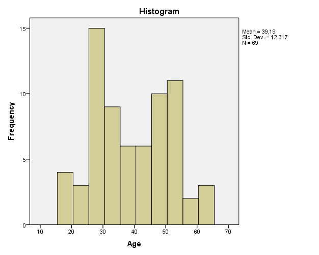
| Age | |||||
| Frequency | Percent | Valid Percent | Cumulative Percent | ||
| Valid | 18 | 2 | 2,9 | 2,9 | 2,9 |
| 19 | 2 | 2,9 | 2,9 | 5,8 | |
| 21 | 2 | 2,9 | 2,9 | 8,7 | |
| 23 | 1 | 1,4 | 1,4 | 10,1 | |
| 26 | 3 | 4,3 | 4,3 | 14,5 | |
| 27 | 2 | 2,9 | 2,9 | 17,4 | |
| 28 | 3 | 4,3 | 4,3 | 21,7 | |
| 29 | 6 | 8,6 | 8,7 | 30,4 | |
| 30 | 1 | 1,4 | 1,4 | 31,9 | |
| 31 | 4 | 5,7 | 5,8 | 37,7 | |
| 32 | 2 | 2,9 | 2,9 | 40,6 | |
| 33 | 1 | 1,4 | 1,4 | 42,0 | |
| 34 | 1 | 1,4 | 1,4 | 43,5 | |
| 35 | 1 | 1,4 | 1,4 | 44,9 | |
| 37 | 2 | 2,9 | 2,9 | 47,8 | |
| 38 | 1 | 1,4 | 1,4 | 49,3 | |
| 39 | 1 | 1,4 | 1,4 | 50,7 | |
| 40 | 2 | 2,9 | 2,9 | 53,6 | |
| 42 | 2 | 2,9 | 2,9 | 56,5 | |
| 43 | 3 | 4,3 | 4,3 | 60,9 | |
| 45 | 1 | 1,4 | 1,4 | 62,3 | |
| 46 | 2 | 2,9 | 2,9 | 65,2 | |
| 47 | 1 | 1,4 | 1,4 | 66,7 | |
| 48 | 5 | 7,1 | 7,2 | 73,9 | |
| 50 | 2 | 2,9 | 2,9 | 76,8 | |
| 51 | 1 | 1,4 | 1,4 | 78,3 | |
| 52 | 2 | 2,9 | 2,9 | 81,2 | |
| 53 | 4 | 5,7 | 5,8 | 87,0 | |
| 54 | 2 | 2,9 | 2,9 | 89,9 | |
| 55 | 2 | 2,9 | 2,9 | 92,8 | |
| 57 | 1 | 1,4 | 1,4 | 94,2 | |
| 59 | 1 | 1,4 | 1,4 | 95,7 | |
| 61 | 1 | 1,4 | 1,4 | 97,1 | |
| 62 | 1 | 1,4 | 1,4 | 98,6 | |
| 63 | 1 | 1,4 | 1,4 | 100,0 | |
| Total | 69 | 98,6 | 100,0 | ||
| Missing | 0 | 1 | 1,4 | ||
| Total | 70 | 100,0 | |||
2.“What proportion of employees belongs to each ethnic group? (Use, for example, Bar Graph)”
FREQUENCIES VARIABLES=ethnicgp
/STATISTICS=RANGE MEAN
/GROUPED=ethnicgp
/BARCHART FREQ
/ORDER=ANALYSIS.
Frequencies
[DataSet1] C:UsersucerDesktop188375_jss.sav
| Statistics | ||
| Ethnic Group | ||
| N | Valid | 70 |
| Missing | 0 | |
| Mean | 1,74 | |
| Range | 3 | |
| Ethnic Group | |||||
| Frequency | Percent | Valid Percent | Cumulative Percent | ||
| Valid | white | 36 | 51,4 | 51,4 | 51,4 |
| asian | 18 | 25,7 | 25,7 | 77,1 | |
| west indian | 14 | 20,0 | 20,0 | 97,1 | |
| african | 2 | 2,9 | 2,9 | 100,0 | |
| Total | 70 | 100,0 | 100,0 | ||
3.“What is the average income? (Use, for example, Descriptive Statistics, Descriptives)”
DESCRIPTIVES VARIABLES=income
/STATISTICS=MEAN STDDEV MIN MAX.
Descriptives
[DataSet1] C:UsersucerDesktop188375_jss.sav
| Descriptive Statistics | |||||
| N | Minimum | Maximum | Mean | Std. Deviation | |
| Income | 68 | 5900 | 10500 | 7819,12 | 997,947 |
| Valid N (listwise) | 68 | ||||
4.“How is number of years worked related to salary, if at all? (Use, for example, Linear Regression)”
REGRESSION
/MISSING LISTWISE
/STATISTICS COEFF OUTS CI(95) R ANOVA
/CRITERIA=PIN(.05) POUT(.10)
/NOORIGIN
/DEPENDENT income
/METHOD=ENTER years.
Regression
[DataSet1] C:UsersucerDesktop188375_jss.sav
| Variables Entered/Removeda | |||
| Model | Variables Entered | Variables Removed | Method |
| 1 | Years Workedb | . | Enter |
| a. Dependent Variable: Income | |||
| b. All requested variables entered. | |||
| Model Summary | ||||
| Model | R | R Square | Adjusted R Square | Std. Error of the Estimate |
| 1 | ,340a | ,115 | ,102 | 945,711 |
| a. Predictors: (Constant), Years Worked | ||||
| ANOVAa | ||||||
| Model | Sum of Squares | df | Mean Square | F | Sig. | |
| 1 | Regression | 7696787,937 | 1 | 7696787,937 | 8,606 | ,005b |
| Residual | 59028359,122 | 66 | 894369,078 | |||
| Total | 66725147,059 | 67 | ||||
| a. Dependent Variable: Income | ||||||
| b. Predictors: (Constant), Years Worked | ||||||
| Coefficientsa | ||||||||
| Model | Unstandardized Coefficients | Standardized Coefficients | t | Sig. | 95,0% Confidence Interval for B | |||
| B | Std. Error | Beta | Lower Bound | Upper Bound | ||||
| 1 | (Constant) | 7410,810 | 180,346 | 41,092 | ,000 | 7050,737 | 7770,883 | |
| Years Worked | 31,841 | 10,854 | ,340 | 2,934 | ,005 | 10,170 | 53,511 | |
| a. Dependent Variable: Income | ||||||||
5. “How different are the average salaries of the different skill categories? (Use, for example, One-way ANOVA)”
ONEWAY income BY skill
/POLYNOMIAL=1
/STATISTICS DESCRIPTIVES
/MISSING ANALYSIS
/POSTHOC=TUKEY ALPHA(0.05).
Oneway
[DataSet1] C:UsersucerDesktop188375_jss.sav
| Descriptives | ||||||||
| Income | ||||||||
| N | Mean | Std. Deviation | Std. Error | 95% Confidence Interval for Mean | Minimum | Maximum | ||
| Lower Bound | Upper Bound | |||||||
| unskilled | 14 | 7628,57 | 730,046 | 195,113 | 7207,06 | 8050,09 | 6500 | 8800 |
| semi-skilled | 18 | 7288,89 | 741,135 | 174,687 | 6920,33 | 7657,45 | 5900 | 8800 |
| fairly skilled | 20 | 8095,00 | 931,029 | 208,185 | 7659,26 | 8530,74 | 6200 | 9500 |
| highly skilled | 16 | 8237,50 | 1267,478 | 316,869 | 7562,11 | 8912,89 | 6400 | 10500 |
| Total | 68 | 7819,12 | 997,947 | 121,019 | 7577,56 | 8060,67 | 5900 | 10500 |
| ANOVA | |||||||
| Income | |||||||
| Sum of Squares | df | Mean Square | F | Sig. | |||
| Between Groups | (Combined) | 9891797,852 | 3 | 3297265,951 | 3,713 | ,016 | |
| Linear Term | Unweighted | 5288030,013 | 1 | 5288030,013 | 5,955 | ,017 | |
| Weighted | 6062905,680 | 1 | 6062905,680 | 6,827 | ,011 | ||
| Deviation | 3828892,173 | 2 | 1914446,086 | 2,156 | ,124 | ||
| Within Groups | 56833349,206 | 64 | 888021,081 | ||||
| Total | 66725147,059 | 67 | |||||
Post Hoc Tests
| Multiple Comparisons | ||||||
| Dependent Variable: Income | ||||||
| Tukey HSD | ||||||
| (I) rated skill | (J) rated skill | Mean Difference (I-J) | Std. Error | Sig. | 95% Confidence Interval | |
| Lower Bound | Upper Bound | |||||
| unskilled | semi-skilled | 339,683 | 335,804 | ,743 | -546,12 | 1225,48 |
| fairly skilled | -466,429 | 328,377 | ,491 | -1332,63 | 399,78 | |
| highly skilled | -608,929 | 344,864 | ,299 | -1518,62 | 300,77 | |
| semi-skilled | unskilled | -339,683 | 335,804 | ,743 | -1225,48 | 546,12 |
| fairly skilled | -806,111 | 306,163 | ,051 | -1613,72 | 1,50 | |
| highly skilled | -948,611* | 323,784 | ,024 | -1802,70 | -94,52 | |
| fairly skilled | unskilled | 466,429 | 328,377 | ,491 | -399,78 | 1332,63 |
| semi-skilled | 806,111 | 306,163 | ,051 | -1,50 | 1613,72 | |
| highly skilled | -142,500 | 316,073 | ,969 | -976,25 | 691,25 | |
| highly skilled | unskilled | 608,929 | 344,864 | ,299 | -300,77 | 1518,62 |
| semi-skilled | 948,611* | 323,784 | ,024 | 94,52 | 1802,70 | |
| fairly skilled | 142,500 | 316,073 | ,969 | -691,25 | 976,25 | |
| *. The mean difference is significant at the 0.05 level. | ||||||
Homogeneous Subsets
| Income | |||
| Tukey HSDa,b | |||
| rated skill | N | Subset for alpha = 0.05 | |
| 1 | 2 | ||
| semi-skilled | 18 | 7288,89 | |
| unskilled | 14 | 7628,57 | 7628,57 |
| fairly skilled | 20 | 8095,00 | 8095,00 |
| highly skilled | 16 | 8237,50 | |
| Sig. | ,074 | ,252 | |
| Means for groups in homogeneous subsets are displayed. | |||
| a. Uses Harmonic Mean Sample Size = 16,703. | |||
| b. The group sizes are unequal. The harmonic mean of the group sizes is used. Type I error levels are not guaranteed. | |||
6. “Is there a significant difference between the proportion of males and females who attended the firm’s meeting last month? (Use, for example, Chi-Squared)”
CROSSTABS
/TABLES=gender BY attend
/FORMAT=AVALUE TABLES
/STATISTICS=CHISQ PHI
/CELLS=COUNT ROW COLUMN TOTAL
/COUNT ROUND CELL.
Crosstabs
[DataSet1] C:UsersucerDesktop188375_jss.sav
| Case Processing Summary | ||||||
| Cases | ||||||
| Valid | Missing | Total | ||||
| N | Percent | N | Percent | N | Percent | |
| Gender * attended meeting | 70 | 100,0% | 0 | 0,0% | 70 | 100,0% |
| Gender * attended meeting Crosstabulation | |||||
| attended meeting | Total | ||||
| yes | no | ||||
| Gender | male | Count | 21 | 18 | 39 |
| % within Gender | 53,8% | 46,2% | 100,0% | ||
| % within attended meeting | 58,3% | 52,9% | 55,7% | ||
| % of Total | 30,0% | 25,7% | 55,7% | ||
| female | Count | 15 | 16 | 31 | |
| % within Gender | 48,4% | 51,6% | 100,0% | ||
| % within attended meeting | 41,7% | 47,1% | 44,3% | ||
| % of Total | 21,4% | 22,9% | 44,3% | ||
| Total | Count | 36 | 34 | 70 | |
| % within Gender | 51,4% | 48,6% | 100,0% | ||
| % within attended meeting | 100,0% | 100,0% | 100,0% | ||
| % of Total | 51,4% | 48,6% | 100,0% | ||
| Chi-Square Tests | |||||
| Value | df | Asymp. Sig. (2-sided) | Exact Sig. (2-sided) | Exact Sig. (1-sided) | |
| Pearson Chi-Square | ,206a | 1 | ,650 | ||
| Continuity Correctionb | ,045 | 1 | ,831 | ||
| Likelihood Ratio | ,206 | 1 | ,650 | ||
| Fisher’s Exact Test | ,810 | ,416 | |||
| Linear-by-Linear Association | ,203 | 1 | ,652 | ||
| N of Valid Cases | 70 | ||||
| a. 0 cells (0,0%) have expected count less than 5. The minimum expected count is 15,06. | |||||
| b. Computed only for a 2×2 table | |||||
| Symmetric Measures | |||
| Value | Approx. Sig. | ||
| Nominal by Nominal | Phi | ,054 | ,650 |
| Cramer’s V | ,054 | ,650 | |
| N of Valid Cases | 70 | ||
The empirical evidence shows that there is scanty of research that investigates the experience of women with reference to Pakistan context. The uniqueness of the Pakistan is their interplay between family structure religion, culture, and class, which affects their reconciliation of family roles and works among Pakistani women. The study uses the in-depth semi-structured interview to investigate the experience of Pakistani women with reference to work-family conflict. The study uses the qualitative data analysis to enhance data reliability and validity. The analysis is carried out by reading the texts to understand the entire context of the interviews.
The outcome of the analysis produces several themes. The first theme produced from the interview is the joint family. It is revealed from the interview that joint family is an essential part of the Pakistani culture. (Anthias, 2013). In Pakistan, all family member sees themselves as one. For example, if one of the family members gets sick, all the family members will rally round the person and take care of him or her. If a woman falls sick, it is a member of the family who will do all the caring while her husband does nothing. The shortcoming of the joint family is that it is impossible for a woman to buy something for herself alone, she is obliged to buy the item for all the member of the family. Moreover, a woman in the joint family cannot buy things for her children alone, she is obliged to buy the same item for all member of the family. (Ammons, . & Edgell, 2007).
Another theme identified in the study is a conflict between a woman role in the family and work. In the Pakistani context, woman expectation is to perform the family roles with regards to the family expectation. While a woman in Pakistan might have worked long hours, the office work responsibility should not affect the childcare and domestic responsibilities. (Anwar, & Shahzad, 2011). For example, the society will judge a woman based on the level of her family caring responsibility. Thus, Pakistani women are expected to fulfill all homemaking no matter her position in her place of work. (Ali et al., 2011). Since women are required to perform both the role of a good woman and ideal worker, inability to perform these roles will be considered a sign of deficiencies. (Arif, & Amir, 2008). For example, women are responsible take care of their husband such as making the breakfast ready, iron their clothes and get everything ready that the husband will need for the office hour the next day. A woman has to fulfill these roles even if she works. Based on the load of work that women are required to carry out in the matrimonial home, 95% of women are happy that they are not working.
Another theme in the study is that men in Pakistan women are not obliged to work and it is men who are to work and take care of the family. One of the participants confirmed this assertion when she was complaining that she had a backache because the office seats are not comfortable, and they are required working non-stop sitting “for long hours on the same chair without any break”. The husband replies: “Leave the job and rest at home. I am not demanding. I never demanded anything from him at all”. The participant also confirms that women need to seek permission from her husband before being allowed to spend their earning. (Ansari, 2011).
A relationship between the Pakistani women and their husband’s relatives is another theme identified in the study because a woman is required to become obstinate for the relative of her husband. In short, women consider men to be the head of the family in Pakistan and women are required to seek for permissions for everything from their husbands. Moreover, the mentality of the husband is to be the only person who is to contribute financially and women are not allowed to contribute financially. One of the participants confirms this assertion by stating:
“When I was at my home, at the time of emergency, birthdays, anniversaries, I used to contribute financially and bought gifts to please my family members. Even I cannot buy a gift for him. My husband tells me to buy things for him from his money. He is not developing a habit of taking money from me. . If a husband starts to take money from his wife, then the wife eventually ends up surrendering before him”.
We hope this example Quantitative and Qualitative Data Analysis essay will provide you with a template or guideline in helping you write your own paper on this topic. You are free to use any information, sources, or topics, titles, or ideas provided in this essay as long as you properly cite the information in your paper and on your reference page.
Ali, T. S. (2011). Living with violence in the home: Exposure and experiences among married women, residing in urban Karachi, Pakistan. Ph.D. Dissertation Department Of Public Health Sciences, Karolinska Institutet, Stockholm, Sweden.
Ammons, S. K. & Edgell, P. (2007). Religious Influences on Work–Family Trade-Offs. Journal of Family Issues, 28(6). 794-826.
Ansari, S. A. (2011). Gender difference: Work and family conflicts and family-work conflicts. Pakistan Business Review, 13(2). 315-331.
Anthias, F. (2013). Intersectional what? Social divisions, intersectionality and levels of analysis. Ethnicities, 13(1). 3-19.
Anwar, M. & Shahzad, K. (2011). Impact of Work-Life Conflict on Perceived Employee Performance: Evidence from Pakistan. European Journal of Economics, Finance and Administrative Sciences, 13(2011). 82-86.
Arif, N. & Amir, T. (2008). Adjustment of Married Working Women in Joint Family System. MA Gender Studies Dissertation Department of Gender Studies, University of the Punjab, Pakistan.
Appendix 1: Data Presentation
Appendix 2 : Variable Presentation